Go to Maple and use the commands  below to convince yourself of the homotopy between a circle and an ellipse.  At the end make sure that you play the animation :

> with(plots):

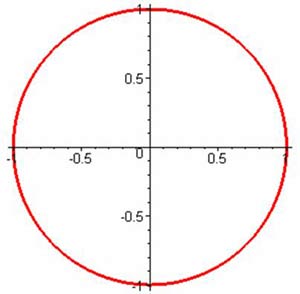
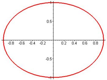
> X1t:=cos(t);

Y1t:=sin(t);

> circle:=plot([X1t,Y1t,t=0..2*Pi],

> scaling=constrained,

           thickness=3,numpoints=200):

> circle;

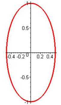
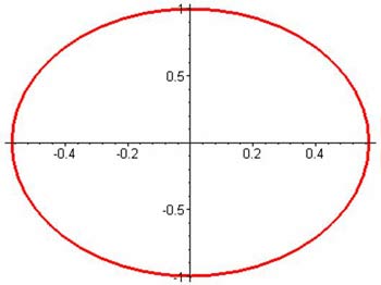
> X2t:=(1/2)*cos(t);

Y2t:=sin(t);

> ellipse:=plot([X2t,Y2t,t=0..2*Pi],

> scaling=constrained,

           thickness=3,numpoints=200):

> ellipse;

Since we used the same interval 0<t<2Pi for both curves, it  is simple to define a homotopy as a linear (convex!) combination of the two curves:

> Xt:=(1-s)*X1t+s*X2t;

Yt:=(1-s)*Y1t+s*Y2t;

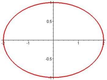
We plot a few intermediate curves: When s is small (near zero) the curve

is "close" to the original curve, when s is large (near one) the curve is close to the

final curve, and some interesting curves  appear in between.

> plot(subs(s=0.1,[Xt,Yt,t=0..2*Pi]),thickness=3);

plot(subs(s=Pi,[Xt,Yt,t=0..2*Pi]),thickness=3);

plot(subs(s=6,[Xt,Yt,t=0..2*Pi]),thickness=3);

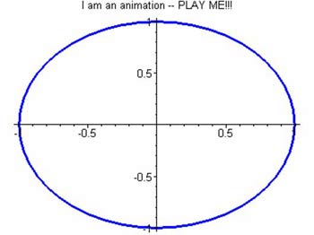
 Ultimately we have a continuous homotopy.  Just for fun, we change the colors and loop it back and forth;

> N:=20;

display([seq(

      plot(subs(s=k/N,[Xt,Yt,t=0..2*Pi]),

           thickness=3,scaling=constrained,

           color=COLOR(RGB,k/N,0,1-k/N)),

         k=[seq(i,i=0..N),seq(N-i,i=0..N)])],

      title=`I am an animation -- PLAY ME!!!`,

      insequence=true);